Broadband service adoption analysis using spatial regression models

Research Question

In this assignment, we are working with the regression model from Assignment 2. In that test, we looked at the regression of various independent variables, and how much variation they explained in our dependent variable, “adopt05”, or the percent of broadband adoption in 2004 among our sample. With these models, we were able to find which independent variables likely explain more of the variability in broadband adoption among the wider population. We also found the measurements of the residuals of these measures, or the portion of the variance that was not explained. What we were not able to do is determine whether there is any spatial dependence that might contribute to the residual unexplained variance.

When measuring spatial autocorrelation, we are looking at whether a particular measure is more similar to that same measure in close proximity than it is to that measure at a further distance. In other words, are similar values clustered together, or are they distributed randomly? One way to determine whether a measure is clustered or random is by using Moran’s I. Then in order to test the significance of those clusters, we need to use other a test that compares the value of Moran’s I to what we would expect if the values are random, or simulations of random data in order to see how likely it is that we would get the value of Moran’s I if the values are random.

Measures

The regression model I chose from the previous assignment, which I was curious about, is that of broadband adoption by median age per county. It wasn’t the strongest measure in the regression model, but I wondered if there was significant spatial clustering of the dependent variable that could be explained by the spatial distribution of median age. The dependent variable is measuring the responses from a survey that indicate broadband adoption in 2004. Using that sample, we can infer the proportion of broadband adoption in the broader population. The independent variable is the median age of the county in 2004. The median age is the age at the middle of the population’s distribution, not the mean or average, which could be skewed by a few very young or very old outliers. My hypothesis is that there is a spatial correlation between an older population and less broadband adoption. This would be an inverse correlation, that as the median age increases, broadband adoption decreases.

Methods

In order to test spatial autocorrelation, we first need to create a network to define who the spatial neighbors are for this comparison. In this analysis, we are defining neighbor’s using the rook’s case, or those which share a boundary, but not a corner. After we define who the neighbors are, we can create a spatial weights matrix, which determines the weight of influence those neighbors have based on the total number of numbers. Once the spatial weights matrix is created by assigning a 1 to each neighbor, a 0 to each non-neighbor, and then dividing the 1 by the number of neighbors, the lagged means can be calculated. These are calculated by multiplying the observed value of each neighbor by that neighbor’s weighted value. Each county then has a lagged mean of its neighbors. That can be compared to the value of the county itself, to see what the relationship is. In this way, first we will test for spatial dependency in the dependent variable, “adopt05”. Then we will use the models of lagged means and the spatial error to test the regression model of “adopt05” by “medage”. Where the Moran’s I can give an indication of clustering or not, it cannot provide the diagnostic of significance. The Monte Carlo test will compare the Moran’s I output to that of complete spatial randomness, 10,000 times, in order to see what the probability is that we would see the value of Moran’s I that we see if the values are random. We can use the Local Moran’s I to understand the clustering of particular high or low values.
If we see a statistically significant Monte Carlo test, we can determine that it is very unlikely that the spatial distribution is random. Rather, we could say with a fairly high certainty that there the values of our dependent variable are affected by their neighbors. That value is represented by the rho value in the result of our spatial autoregression model.

Results

• 

• 

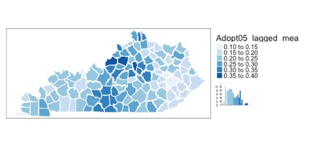
The map above shows how much influence the lagged means, or the weights of the neighbors times their value for “adopt05” exert on the dependent variable of each county. There seems to be a much stronger spatial influence in the central parts of the state, especially in the north central areas. From what we saw in the map of the dependent variable above, it seems that the areas where the percent of broadband adoption is greater also have large influence on their neighbors. Considering the physical infrastructure necessary to expand broadband networks, it isn’t surprising that the places where it is found are clustered together. Whether that clustering is significant and not random will be shown in the Monte Carlo simulation of our Moran’s I model.

Global Moran’s I for regression residuals

Model: lm(formula = reg.eq1, data = KYMap)
Weights: listw1

Moran I statistic standard deviate = 4.1204, p-value = 0.00001891
Alternative hypothesis: greater
Sample estimates:
Observed Moran I Expectation Variance
0.226727978 -0.010564525 0.003316559

The global Moran’s I measures global spatial association by analyzing the region as a whole. The test can tell us if there is clustering, by giving the observed Moran’s value vs the expected. However this in itself cannot tell where the clustering is happening, or how significant the clusters are.

Monte-Carlo simulation of Moran I

Data: KYMap$adopt05
Weights: rook_listw
Number of simulations + 1: 10001

Statistic = 0.25606, observed rank = 10001, p-value = 0.00009999
Alternative hypothesis: greater

By running 10000 additional simulations that randomize the data, we are able to see that the likelihood we would achieve the observed Moran’s I value that we found if the data were random is much less than .05% (p-value = 0.00009999). This means the clustering found here is statistically significant, and not random.

Conclusion:

After analyzing the regression model of “adopt05” by “medage” in a spatial autoregression model, I would infer because there is statistically significant spatial clustering of our dependent value and significant influence of the independent measure upon the dependent measure in our model, that we would be very likely to find that in the general population across these areas. However, it does not seem to explain as large of a portion of the variability, or exert as strong of an influence as I thought it might from the original regression model. I would like to explore other variables such as other levels of physical infrastructure in a spatial model, such as the percent of paved roads, or perhaps the infrastructure of municipal utilities offered. I would also like to add the variable of race and ethnicity, to see if there is an inequality of services offered by race.