Research Question
When we take some measurements at certain points, we might want to know what would be the likely values in areas where we don’t have any points measured. We use interpolation to find the answer to that question. Interpolation addresses a second order process. The difference between first order and second order point pattern analysis is the relationship between points. In a first order process, we are assuming that there is an equal chance for the points to occur anywhere in our geographic area. This assumption is based on the independence of points from each other. However, in a second order process we are not assuming the points are independent of one another. Instead, we are assuming that if we have one point of a certain value, there is a great chance of having other points nearby of a similar value, than in other areas. Therefore, our null hypothesis is that our points do not exert any influence on the points around them, and we expect to see a totally random distribution of values, or complete spatial randomness (CSR)
Below we analyze the methods and results of Nearest Neighbor and Inverse Distance Weighting analyses, and offer an overview of another method, Kriging. The first two do not include any way of estimating the error or probability of these measurements. Nearest Neighbor and Inverse Distance Weighting are based on distance or area and are purely deterministic analyses. Kriging not only makes estimates for the measurements in between points, but also provides an estimate of error for those points. Kriging uses a spatial statistical analysis for the points it is estimating, offering a probabilistic method for estimating points and the error in those values.
Measures
Our points come from 2015 greenhouse gas emissions from EPA monitored sites, where each site has a listing for their emissions in carbon metric tons. There are 89 sites with emissions readings between 0 and 4,184,267. Interestingly, the refinery that just caught fire this weekend is the second highest emitter of greenhouse gases, at 3,110,037 carbon metric tons and narrowly missed a dangerous release of hydrofluoric acid during this most recent fire. Our study area includes the four Mid-Atlantic states – Pennsylvania, Delaware, New Jersey, and Maryland. Most of the points we have readings for are along the Delaware River and surrounding areas.
Nearest Neighbor
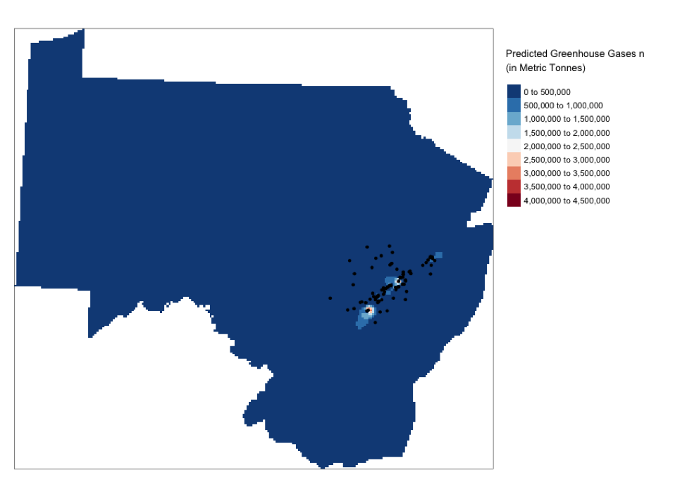
In the analysis below, the region has been tessellated into regions related to the point they are closest to. These areas are called Thiessen polygons, and the areas closest to the points are smaller as the mean distance between the points is much smaller, where the areas around the edges essentially have a mean going to infinity, since we don’t have another known point with which to calculate a mean with. After the Thiessen polygons are created, we mask the surface with our states area, so that we can gain the values for the geographic area we are looking at. Then by measuring the distance to our measured value, Nearest Neighbor estimates a value for the unmeasured points. Below we can see the small areas closest to the points that have slightly higher estimated values, but the vast majority of our area has so few points and is so far from the points measured that the predicted greenhouse gas emissions is almost none.

Inverse Distance Weighting
In this method, a raster grid is created that covers the area we want to estimate values for. Then using a formula of inverse distance from our points, each square of the grid has a value estimated based on the known points. However, it is assumed that each predicted value is influenced more by points closer to it than points further away. This function is affected by what power of inverse relationship is used, with a faster decay rate at a power of 4 than a power of 2, for example. Like Nearest Neighbor, this isn’t probabilistic and therefore the likelihood of the estimates can’t be measured. The accuracy must be determined by taking more measurements.
Regression of coordinates
Is there a significant relationship between the data and the geographical coordinates? No, the p-value is not significant, so we can’t say that geography alone is predictive of the changes in metric tonnes of carbon.
Residuals:
Min 1Q Median 3Q Max
-568071 -326112 -224745 -42966 3719087
Coefficients:
Estimate Std. Error t value Pr(>|t|)
(Intercept) 25208998.428 19042456.307 1.324 0.189
ghg$X 2.039 3.587 0.568 0.571
ghg$Y -5.853 4.508 -1.298 0.198
Residual standard error: 710500 on 86 degrees of freedom
Multiple R-squared: 0.0195, Adjusted R-squared: -0.003306
F-statistic: 0.855 on 2 and 86 DF, p-value: 0.4289

Plot of points in UTM 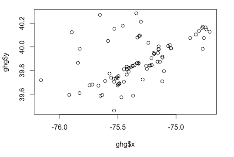
Plot of points in WGS
Kriging
The final method tested but not completed here is Kriging, which combines deterministic and probabilistic methods to measure the geographic distribution, as well as the spatially correlated and uncorrelated points. Kriging finds a mathematical function based on the statistical relationship of the points that are known. It is based on the idea of spatial autocorrelation, that points nearer to each other in space are more similar. The difference or mean of each pair of points is measured in relation to their distance apart. When difference and the distance are plotted it forms a semivariogram. When spatial autocorrelation is occurring, function will increase to a point and then flatten out to a “sill”. The increasing portion of the function is the “range” in which the values relate to one another, and the flat portion is where the relationship between points diminishes or ends. The intercept is called the “nugget” – this is the point where the measurements are a result of spatial noise, and are spatially independent.
In Kriging, we are able to not only analyze the function of distance, but also the function of difference between points, and apply statistical model. Because it uses a statistical model, it also generates an error measure, or how much our estimate is missing the mark.
Conclusion
Based upon the measurements we have, I do believe that Kriging would apply the best method, not simply because it offers the error estimate, but because it doesn’t rely only on a distance or weighting method. We are dealing with a measurements that vary extremely widely, and it would be helpful to see the relationship between those points and the areas around them in a way that offers more ways to test our predictions. Air quality measurement is difficult to grasp in a geographic analysis because of the limited number of sensors and limited number of measurements taken for a variety of airborne pollutants. Just as this most recent refinery explosion was explained as not harmful, what exactly was burning and how that was directly affecting air quality was not immediately shared. When a facility has a track record of high emissions, it would be helpful to analyze the probability of areas around it having high exposure to those emissions. Even if we can estimate those measurements by distance, we need a more concrete way to test those measurements and offer health and safety analyses for the residents and workers most exposed to these gasses.

You must be logged in to post a comment.